Big O

Big O is the metric we use to describe the efficiency of algorithms. When developing algorithms, a lack of high level understanding of Big O can really hurt. Writing code that can scale is important, understanding Big O helps in that objective.

Ignoring a more academic understanding of Big O, it is commonly considered to be the measurement of how run time and spacetime grow as the input to an algorithm grows. This definition allows us to talk about algorithms agnostic of the machines they run on. We are not measuring how fast an algorithm will run on any given machine, we are instead measuring what will happen to an algorithm when the input size into it grows. This helps us understand if what we build will scale.

To better understand Big O, it helps to start with an intuitive example. Lets consider a function to search for a key in a list of integers. We first can try a linear search that loops through the list and compares each value against the key:

1bool linear_search(const std::vector<int> &vals, int key) noexcept {
2    for (const auto& v : vals) {
3        if (v == key) {
4            return true;
5        }
6    }
7    return false;
8}

The runtime Big O for this function would be O(n) where n is the size of the vector being passed in. This is because we always consider the worst case scenario when determing the runtime. The key might be the last value in the vector which means we must iterate over each item in the vector before finding our key. This has a linear runtime, the runtime will grow proportional to the input size. But next lets consider a binary search function:

 1bool binary_search(const std::vector<int> &vals, int key) noexcept {
 2    int start = 0, end = vals.size() - 1;
 3    while (start < end) {
 4        int mid = (start + end) / 2;
 5        if (vals[mid] == key) {
 6            return truel
 7        } else if (vals[mid] < key) {
 8            start = mid + 1;
 9        } else {
10            end = mid - 1;
11        }
12    }
13    return false;
14}

Here, with every iteration over the while loop, we half the amount of the vector we need to consider. The runtime Big O for this function is O(log n). The difference between these two functions is negligible for small inputs, but massive as the input grows. On an input of 64 items, the linear search might need to look through all 64 items. But at most, the binary search will need to look through 7 items. What if we double the input to 128 items? The linear search now doubles its runtime, but the binary search now only needs to iterate the while loop 8 times at most instead of 7. This means the binary search will scale significantly better than the linear search.

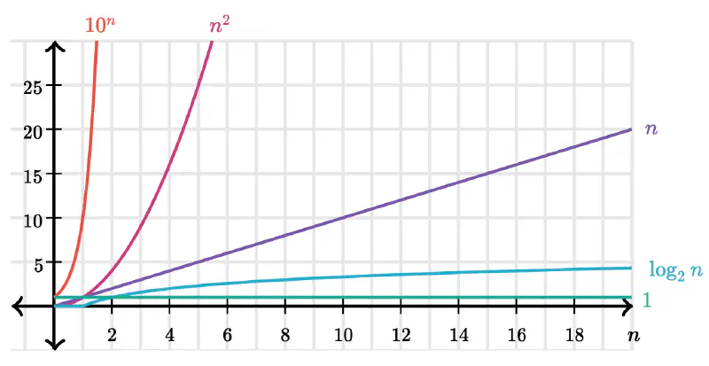
Some of the most common growth rate functions a developer is expected to see are:

O(1) - constant time O(log n) - logarithmic time O(n) - linear O(n log n) - linearithmic O(n^2) - quadratic O(2^n) - exponential

This is a cool chart that helps visualize these growth rates:

Ok - lets do some examples to help glue this altogether.

What is the runtime of this function:

 1void foo(const std::vector &array) noexcept {
 2    int sum = 0;
 3    int production = 1;
 4    for (int i = 0; i < array.size(); i++) {
 5        sum += array[i];
 6    }
 7    for (int i = 0; i < array.size(); i++) {
 8        product *= array[i];
 9    }
10    std::cout<<sum<<", "<<product;
11}

O(n). It does not matter that we loop through the vector twice. We are measuring the rate of growth which is not impacted by running through the array twice independent of each other. Theoretically the Big O would be O(2n). But in Big O, we remove constants, so it would only be O(n).

What is the runtime of this function:

1void printPairs(const std::vector &array) noexcept {
2    for (int i = 0; i < array.size(); i++) {
3        for (int j = 0; j < array.size(); j++) {
4            std::cout<<array[i]<<", "<<array[j];
5        }
6    }
7}

O(n^2). The inner loop O(n) is run n times because of the outter loop.

What is the runtime of this function:

1void printPairs(const std::vector &array) noexcept {
2    for (int i = 0; i < array.size(); i++) {
3        for (int j = i + 1; j < array.size(); j++) {
4            std::cout<<array[i]<<", "<<array[j];
5        }
6    }
7}

O(n^2). This one is less intuitive because each inner loop is decreasing in size compared to its previous iteration. Lets break this down. The inner loop will run: (n - 1) + (n - 2) + (n - 3) .. = 1 + 2 + 3 + … n - 1 = n(n - 1) / 2 = n^2 / 2 = in BigO, we remove the constants which means we got n^2. Despite the algorithm only searching what will be half of the entire pairs, the rate of growth remains quadratic.

An example that can trip people up is if we take the last function but modify it to be two arrays instead:

1void printPairs(const std::vector &array1, const std::vector &array2) noexcept {
2    for (int i = 0; i < array1.size(); i++) {
3        for (int j = i + 1; j < array2.size(); j++) {
4            std::cout<<array[i]<<", "<<array[j];
5        }
6    }
7}

Many would think this is still O(n^2) since it it almost identical to the example above. But it must be remembered that we are measuring runtime growth based on input size. In this case, there are two inputs and both matter. The actual runtime is O(ab), where a is array1 and b is array2.

Recursive Patterns Computing the BigO of a recursive function is typically O(branches^depth). A classic example is the Fibinacci sequence:

1int fib(int n) {
2    if (n <= 0) { 
3        return 0; 
4    } else if (n == 1) {
5        return 1;
6    }
7    return fib(n - 1) + fib(n - 2)
8}

Here we have two branches (recursive calls in the last line of the function) and the depth will be n since we call until we decrement to 1 or 0. So our BigO is O(2^n).

The examples get a lot more tricky when the algorithms get more complex. Here is an example that has often tripped me up:

• Suppose we have an algorithm that took in an array of strings, sorted each string, and then sorted the full array. What would the runtime be?

Answering this involves breaking this up into smaller chunks.

1. First we need to loop through each string and sort it. Sorting a string will take O(s log s), but we need to sort each string so make it a * s log s where a is the length of the array.
2. Now we have to sort all the strings that have each been sorted. Sorting strings is a challenge since you will need to compare each string with takes O(s) for each comparison. Since sorting takes O(a log a), that notation also represents how many comparisons you need to make with each comparison taking O(s).Therefore this step will take O(a * s log a). This makes sense when you think about it. For a normal sort of something like a vector of integers, a comparison between two values is done in one step which is a constant you can remove from the notiation. In this case, the comparison of a string takes O(s) so it must be included in the notation.
3. So we know the first step take O(a * s log s) and the second step takes O(a * s log a). We now need to combine them. The answer is:

= O(a * s log s + a * s log a) You can factor out the a * s log = O(a * s(log s + log a))

The focus here was primarily on runtime. There are a lot of ways BigO can trip you up, but a good understanding will help ensure better programming and our software scales out there in the real world.